Using FDTD

FDTD can be used for varios type of simulations: light scattering from arbitrary shaped objects, modeling of source radiation in specified electromagnetic environment, optical properties of resonators and waveguides. In this section we consider these and other possible examples in details.

Preliminary notes

Solution of Maxwell's equations \({\bf F}({\bf r},t)\) ( \(\bf F\) is \(\bf E\) or \(\bf H\)), in absence of free charges, current sources and any nonlinearities, can be represented as a superposition of harmonic fields:

\( {\bf F}({\bf r},t)={\bf A}({\bf r},\omega)\cos{\omega t}+{\bf B}({\bf r},\omega)\sin{\omega t} \)

It is convenient to look at \({\bf F}\) as a real part of complex vector

\( {\bf F_c}={\bf C}\exp(-i\omega t) \)

where

\( {\bf C}={\bf A}+i{\bf B} \) \( {\bf F}={\rm Re}({\bf F_c}) \)

Complex dependency \(\exp(-i\omega t)\) is introduced for convenience purposes only and does not have any physical meaning.

The Poynting vector \({\bf P} = {\bf E} \times {\bf H}\) specifies the magnitude and direction of the rate of electromagnetic energy transfer. The instantaneous Poynting vector is rapidly varying function of time for frequencies that are usually of interest. Most instruments are not capable of following the rapid oscillations of the instantaneous Poynting vector, but respond to some time average \({\bf S}\):

\( {\bf S}=<{\bf P}>=\frac{1}{\tau}\int_t^{t+T}{\bf P}(\tau) d\tau \)

where \(T\) is a time interval long compared with \(1/\omega\).

It can be shown that for harmonic field

\( {\bf S}=\frac{1}{2}{\rm Re}({\bf E_c}\times{\bf H^*_c}) \)

Light intensity \(I\) is absolute value of \({\bf S}\).

Absorption and scattering by arbitrary object

Consider arbitrary object illuminated by harmonic incident wave. Field in the medium surrounding the object can be represented as superposition of incident and scattered fields:

\( {\bf E}={\bf E_i}+{\bf E_{s}}, \qquad {\bf H}={\bf H_i}+{\bf H_{s}} \)

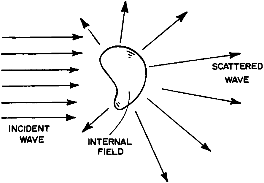
Here we consider how to estimate energy scattered and absorbed by object. We construct imaginary closed surface around the object \(A\); the net rate at which electromagnetic energy crosses this surface is

\( W_{abs}=-\int{\bf S}\cdot{\bf n} dA \)

where \({\bf n}\) is normal to the surface.

If \(W_{abs}>0\), energy is absorbed within the volume confined by surface. If object is embedded in nonabsorbing environment, \(W_{abs}\) is the rate at which energy is absorbed by object.

Time averaged Poynting vector \({\bf S}\) can be represented as (we omit here index \(c\) for complex vectors \({\bf E}\) and \({\bf H}\))

\( {\bf S}=\frac{1}{2}{\rm Re}({\bf E}\times{\bf H^*})={\bf S_i}+{\bf S_{sca}}+{\bf S_{ext}} \)

where

\( {\bf S_i}=\frac{1}{2}{\rm Re}({\bf E_i}\times{\bf H_i^*}), \qquad {\bf S_{sca}}=\frac{1}{2}{\rm Re}({\bf E_{s}}\times{\bf H_{s}^*}), \qquad {\bf S_{ext}}=\frac{1}{2}{\rm Re}({\bf E_i}\times{\bf H_{s}^*}+{\bf E_{s}}\times{\bf H_i^*}) \)

Last term \({\bf S_{ext}}\) is a consequence of an interference between incident and scattered fields.

After integrating over surface we have

\( W_{abs}=W_i-W_{sca}+W_{ext} \) \( W_i=-\int{\bf S_i}\cdot{\bf n} dA, \qquad W_{sca}=\int{\bf S_{sca}}\cdot{\bf n} dA, \qquad W_{ext}=-\int{\bf S_{ext}}\cdot{\bf n} dA \)

For nonabsorbing environment \(W_i=0\), and

\( W_{ext}=W_{abs}+W_{sca}. \)

These energy flow rates are linearly dependent on incident wave intensity \(I\). Their normalized values

\( C_{ext}=\frac{W_{ext}}{I}, \qquad C_{abs}=\frac{W_{abs}}{I}, \qquad C_{sca}=\frac{W_{sca}}{I} \)

are extinction, absorption and scattering cross sections with dimensions of area.

We may define efficiencies for extinction, scattering and absorption

\( Q_{ext}=\frac{C_{ext}}{G}, \qquad Q_{abs}=\frac{C_{abs}}{G}, \qquad Q_{sca}=\frac{C_{sca}}{G} \)

where \(G\) is the object cross-sectional area projected onto a plane perpendicular to the incident beam (e.g. \(G=\pi r^2\) for a sphere of radius \(r\)). Particles can scatter and absorb more light that is geometrically incident upon them (corresponding efficiencies are greater than unity) if their sizes are comparable or smaller than the incident wavelength.

The amplitude scattering matrix

This matrix is used to characterize angular distribution of scattered light.

Consider object that is illuminated by a harmonic wave.

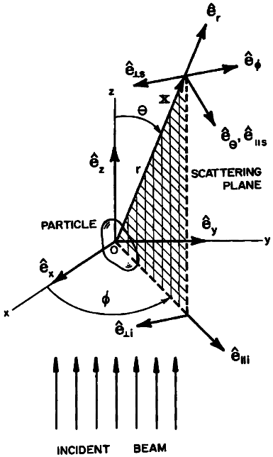
The direction of propagation of the incident light defines \(z\) axis, the forward direction. Any point in object may be chosen as the origin \(O\) of a rectangular coordinate system, where \(x\) and \(y\) axes are orthogonal to \(z\) axis and to each other but otherwise arbitrary. The orthonormal basis vectors \({\bf e_x}\), \({\bf e_y}\), \( {\bf e_z}\) are in direction of positive \(x\), \(y\) and \(z\) axes.

The scattering direction \({\bf e_r}\) and forward direction \({\bf e_z}\) define a scattering plane. This plane is uniquely determined by the azimuthal angle \(\phi\), except when \({\bf e_r}\) is parallel to the \(z\) axis. In this two instances ( \({\bf e_r}=\pm{\bf e_z}\)) any plane containing \(z\) axis is a suitable scattering plane.

It is convenient to resolve the incident electric field \({\bf E_i}\), which lies in the \(xy\) plane, into components parallel and perpendicular to the scattering plane

\( {\bf E_i}=\left( E_{0\parallel}{\bf e_{\parallel{}i}}+E_{0\perp}{\bf e_{\perp{}i}} \right) \exp(i\vec{k}\vec{z}-i\omega{}t)= E_{\parallel{}i}{\bf e_{\parallel{}i}}+E_{\perp{}i}{\bf e_{\perp{}i}} \)

The orthonormal basis vectors

\( {\bf e_{\perp{}i}}=\sin\phi{\bf e_x}-\cos\phi{\bf e_y} \) \( {\bf e_{\parallel{}i}}=\cos\phi{\bf e_x}+\sin\phi{\bf e_y} \)

form a right-handed triad with \({\bf e_z}\):

\( {\bf e_{\perp{}i}}\times{\bf e_{\parallel{}i}}={\bf e_z} \)

We also have

\( {\bf e_{\perp{}i}}=-{\bf e_{\phi}}, \qquad {\bf e_{\parallel{}i}}=\sin\theta{\bf e_r}+\cos\theta{\bf e_{\theta}} \)

where \({\bf e_r}\), \({\bf e_{\theta}}\), \({\bf e_{\phi}}\) are orthonormal basis vectors associated with the spherical polar coordinate system \((r, \theta, \phi)\).

If the x and y components of the incident field are denoted by \(E_{xi}\) and \(E_{yi}\), then

\( E_{\parallel{}i}=\cos\phi{}E_{xi}+\sin\phi{}E_{yi} \) \( E_{\perp{}i}=\sin\phi{}E_{xi}-\cos\phi{}E_{yi} \)

At sufficient distances from the origin ( \({\bf kr}\gg{}1\)), in the far-field region, the scattered field is approximately transverse ( \({\bf e_r} \cdot {\bf E_s} \sim 0 \)) and has the asymptotic form

\( {\bf E_s}=E_{\parallel{}s}{\bf e_{\parallel{}s}}+E_{\perp{}s}{\bf e_{\perp{}s}} \)

where:

\( {\bf e_{\parallel{}s}}={\bf e_{\theta}}, \qquad {\bf e_{\perp{}s}}=-{\bf e_{\phi}}, \qquad {\bf e_{\perp{}s}} \times {\bf e_{\parallel{}s}} = {\bf e_r} \)

The basis vector \({\bf e_{\parallel{}s}}\) is parallel and \({\bf e_{\perp{}s}}\) is perpendicular to the scattering plane. Note, however, that \({\bf E_s}\) and \({\bf E_i}\) are specified relative to different set of basis vectors. Because of the linearity of Maxwell's equations, the relation between them can be written in matrix form

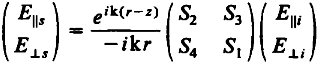
where \(S_j\) ( \(j=1,2,3,4\)) are elements of the amplitude scattering matrix, and depend in general on scattering angle \(\theta\) and azimuthal angle \(\phi\).

Experimental measurement of elements \(S_j\) is difficult. However, the amplitude scattering matrix is related to elements of so called scattering matrix, the measurement of which poses considerable fewer experimental problems. Scattering matrix is real matrix \(4\times{}4\), with 7 independent elements, which can be expressed using absolute values \(\left|S_j\right| (j=1,2,3,4)\) and phase differences between \(S_j\). One can find more detailed information in chapter 3.3 of book (1).

Applications

EMTL was applied for various range of optical applications. Here is chosen publications list:

(1) C. F. Bohren and D. R. Huffman: Absorption and Scattering of Light by Small Particles, Wiley-Interscience, New York (1983)
A. Deinega, I. Valuev, B. Potapkin and Yu. Lozovik, "Minimizing light reflection from dielectric textured surfaces," JOSA A 28, 770 (2011)
S. Zalyubovskiy et. al., "Theoretical limit of localized surface plasmon resonance sensitivity to local refractive index change and its comparison to conventional surface plasmon resonance sensor", JOSA A 29, 994 (2012)
A. Deinega, S. John, "Solar power conversion efficiency in modulated silicon nanowire photonic crystals", J. Appl. Phys. 112, 074327 (2012)
S. Belousov et. al., "Using metallic photonic crystals as visible light sources", Phys. Rev. B 86, 174201 (2012)
A. Deinega, S. Eyderman, S. John, "Coupled optical and electrical modeling of solar cell based on conical pore silicon photonic crystals", J. Appl. Phys. 113, 224501 (2013)