Modeling of the reflection spectrum of a structure with a deposited one-dimensional diffraction grating

High-performance photocathodes have become an advanced technology for modern electron sources and accelerators. Quantum efficiency (QE) is a measure of the photosensitivity of an optical device, it is an important parameter for evaluating the performance of photocathodes. High quantum efficiency makes it possible to obtain high-brightness electrons, reduce heating, extend the service life and increase the energy efficiency of optical devices

To increase QE, nanoscale diffraction gratings are applied to flat photocathodes. Due to this, a plasmon resonance occurs at the photocathode interface, which leads to an increase in the absorption capacity of the structure. The greater the absorption of the structure, the higher the quantum efficiency. Using the FDTD method, reflection spectra can be calculated.

Quantum efficiency and absorption capacity, according to the three-stage Spicer model, are related by the following formula:

\[QE = (1-R)F_{e-e}M, \]

where R is the reflectivity of the structure, \(F_{e-e}\) is the probability of electron transport to the surface, M is the probability of the electron overcoming the output operation. It can be seen that the quantum efficiency is directly proportional to the absorption capacity of the material. Here we will calculate the reflection spectrum from a photocathode with a diffraction grating having a one-dimensional periodicity. Applying such a structure significantly reduces reflection. In addition, we will find the distribution of the field on the interface. We will look for the spectrum in the optical wavelength range from 0.4 to 1.2 micrometers. The structure diagram is made in the "Blender" program, it is presented in (Fig. 1)

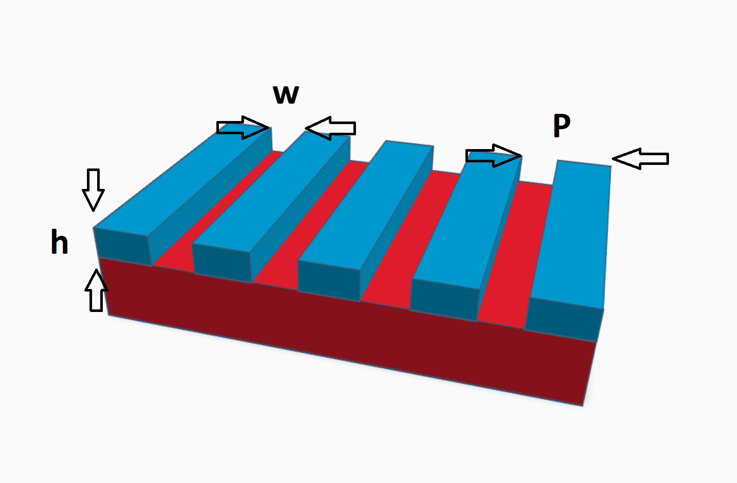
Fig. 1. Geometry of the structure, the following parameters were used for all calculations: \(w = 0.224\), \(p = 0.512\), \(h = 0.032\), all values in micrometers

Let's set the geometric parameters of the model:

w = 0.224
h = 0.032
p = 0.512

Problem statement

The aim of the work is to find the reflection spectrum from a structure with a one-dimensional diffraction grating with an accuracy of 4 nm
The aim is also to find the field distribution near the interface with an accuracy of 4 nm at the frequency at which the greatest absorption is observed.

To do this, you need:

Build the geometry of the problem
Set the dielectric parameters of the material
Install detectors from which simulation results will be output
Visualize the results

Program Description

Preparation for the calculation

To solve this problem, we will use the library EMTL, which is based on the method FDTD. Let's move on to writing the program.

First of all, you need to connect the library:

import emtl

To correctly output the log and files, you need to connect the library "sys" and write the following command:

import sys

emtl.emInit(sys.argv[1:])

The FDTD experiment is carried out using the uiPyExperiment class. You need to create an object of this class, and then call its functions sequentially, with the help of which the geometry of the experiment is set, calculation and subsequent analysis are carried out. Let's create an instance of the class and specify that all results should be output depending on the wavelength:

task = emtl.uiPyExperiment()

For convenience, using the Use Lambda method, we will set the output of the program in micrometers. Now we will set the wavelength range in micrometers in which the spectrum will be calculated using the SetWavelengthRange method. The last two arguments specify the range in micrometers, and the first argument sets the upper limit of the number of points at which the spectrum will be calculated.

task.UseLambda(1)

task.SetWavelengthRange(600, 0.4, 1.2)

Micrometers are considered the standard unit in the program, and time is measured in the speed of light in inverse micrometers. We don't need him yet. Setting spatial accuracy:

dx = 0.004

task.SetResolution(dx, 0.5) #accuracy

The second optional argument of the SetResolution function is the Clock ratio, it is the ratio of the time step to the grid step, the default value for which is 0.5 (with this value, FDTD works steadily).

The computational volume we will have will be a parallelepiped with opposite angles (0, 0, 0) and (p, 0, 2p). The size of 2p along OZ was chosen because there should be a significant distance between the structure and the absorbing boundary conditions. It is also important that the structure under study be removed from the PML

task.SetInternalSpace(emtl.Vector_3(0),emtl.Vector_3(p, 8*dx, 2*p))

Let's set absorbing PML boundary conditions on top and bottom of the computational volume and periodic conditions on the sides of the computational volume.

task.SetBC(emtl.BC_PER, emtl.BC_PER, emtl.BC_PML)

task.SetPMLType(emtl.NPML_TYPE)

We specify the calculation mode "Fourier on fly" using the "SetFourierOnFly" method. This allows you to speed up the program.

task.SetFourierOnFly(True)

Geometry and material definition

How to create geometric bodies is described here. If the bodies go beyond the boundaries of the computational volume, then only the part of them that falls into it is considered.

It is enough to specify an elementary cell of the structure. It consists of a half-space of silver, and a groove cut in it

box = emtl.GetBox(emtl.Vector_3((p-w)/2, 0, p), emtl.Vector_3((p-w)/2+w, 8*dx, p+h)) #
halfspace = emtl.GetHalfSpace(emtl.Vector_3(0, 0, 1),
                                           emtl.Vector_3(0, 0, p))

Using the GetBox method, a parallelepiped geometry is created. The arguments of this method are two vectors of coordinates of points. These points are opposite corners of the parallelepiped. Since the groove is assumed to be unlimited along the OY axis, we specify the length of the parallelepiped along the OY axis equal to 8 dx, that is, coinciding with the length of the computational volume. The GetHalfSpace method allows you to set the geometry of a half-space. Recall that periodic boundary conditions are established along the OY axis. The first argument is the direction vector inside the half-space, and the second argument specifies a point on the interface of the half-space.

FDTD does not imply the possibility of tabulating the dependence of the dielectric constant on the frequency. However, in FDTD, you can set this dependence as an arbitrary number of terms in the form of Drude and Lorentz. We will not dwell in detail on what parameters are set by different members, we will only give their form:

Debye: \(\frac{\Delta\varepsilon}{1-2i\omega\gamma_p}\)
Drude: \(\frac{\Delta\varepsilon\omega_p^2}{-2i\omega\gamma_p-\omega^2}\)
Lorenz: \(\frac{\Delta\varepsilon \omega_p^2}{\omega_p^2-2i\omega\gamma_p-\omega^2}\)
Modified Lorentz: \(\frac{\Delta\varepsilon\left(\omega_p^2 - i\omega\gamma'_p\right)}{\omega_p^2-2i\omega\gamma_p-\omega^2}\)

You can get amateurish information about the frequency in the representations of a Friend-Lorentz earns the sum of people who are friends, Lorentz and Debye. In addition, you can read about this offer here. The parameters for the approximation were obtained using memory approximation programs. The results of the study of the statistics of A.D. Rakich, A. B. Djurisic, J. M. Elazar and M. L. Mayevsky were used for the study. Optical properties of metal films for optoelectronic devices with vertical resonator

import math
 
silver = emtl.emMedium(1.000)
silver.AddPolarizability(emtl.emDrude(0.012782, 0.080051, 5.153889))
silver.AddPolarizability(emtl.emDebye(2.5, 0.123338))
silver.AddPolarizability(emtl.emLorentz(0.000751, 0.080051, 6.573403))
silver.AddPolarizability(emtl.emLorentz(0.003118, 0.000243, -0.227118, 0))
silver.calibrate(2*math.pi*1e3)

You can get amateurish information about the frequency in the representations of a Friend-Lorentz earns the sum of people who are friends, Lorentz and Debye. In addition, you can read about this offer here. The parameters for the approximation were obtained using memory approximation programs. The results of the study of the statistics of A.D. Rakich, A. B. Djurisic, J. M. Elazar and M. L. Mayevsky were used for the study. Optical properties of metal films for optoelectronic devices with vertical resonator

However, many materials are already in the library:

silver = emtl.getAg()

air = emtl.emMedium(1.0)

It remains only to add bodies. Using the level parameter, you can indicate the priority of the body. The higher the value of the level attribute for a body, the higher its priority. If two bodies with different priorities overlap each other, then in the overlap region the dielectric constant will be the same as that of a body with a higher priority. By default, the body is assigned priority 0.

task.AddObject(silver, halfspace)

task.AddObject(air, box, level = 1)

Total Field / Scattered Field

To generate a plane wave, we will use the Total Field/Scattered Field (TF/SF) method. The Total Field area will be located inside the half-space that is above the z = 0.05 plane

task.AddTFSFPlane(emtl.INF, emtl.INF, 0.05)

It is desirable that there should be a distance of at least 1.5 grid steps in space between the body and the TF/SF boundary

As an incident wave used in the Total Field area, we will use a time-limited pulse with a flat front propagating in the direction (0,0,1) and polarized along the direction (1,0,0):

task.SetPlaneWave(emtl.Vector_3(0,0,1), emtl.Vector_3(1,0,0))

Let's set the time dependence of the incident pulse in the Berenger form. As an argument, a class encapsulating a certain signal is sent to the Set Signal() method. It is important to use the emtl.new() method when setting an argument in this way

dx_1 = 0.01

task.SetSignal(emtl.new(emtl.Berenger(1, 25 * dx_1, 10 * dx_1, 125 * dx_1)))

Detectors

In order to measure the fields inside the computational volume, detectors are needed. They read the values of the field at the points where they are placed, without affecting it in any way. The values on the detectors are obtained by interpolation over nearby grid nodes. During the numerical experiment, the detectors record their readings in binary files. Further, readable text files will be created based on these binary files.

The reflection coefficient can be found by dividing the reflected field flux from the structure by the field flux of the incident radiation. You can fix the reflected field flow using the Addraset method, it creates a plane of detectors for this. This method takes four arguments: the first argument is a string, the name of a group of detectors, the second argument is an axis that will be perpendicular to the planes of the detectors (x - 0, y - 1, z – 2), the next two arguments are the coordinate on the previously selected axis through which the detectors of the reflection and transmission field flow pass. Since the structure is supposed to be large enough, it does not miss reflection, so the third argument responsible for the position of the plane of the absorption detectors can be put by anyone. The second argument sets the position of the plane of the detectors reading the reflected stream, so this plane should be in the "Scattered field" area.

task.AddRTASet("flux", 2, 0.025, 0.1, 0.5)

To find the distribution of the field, add detectors using the AddDetectorSet method. The first argument of which is the name of the detector, the next two are the coordinates of the opposite corners of the parallelogram, inside the volume of which the field will be measured. The third argument specifies the number of detectors along a certain coordinate axis, for example, by specifying emtl.iVector_3(128, 1, 32), we specify 128 detector planes along the OX axis, 1 plane along the OY and 32 along the OZ axis. The last argument is a flag and means that the distribution of the field will be measured depending on the frequency, if "emtl.DET_T" was specified, then the field would be removed depending on the time.

#task.AddDetectorSet("frequency", emtl.Vector_3(0, 0, p-2*h), emtl.Vector_3(p, 0, p+2*h), emtl.Vector_3(-1), emtl.DET_F | emtl.DET_BIN_ONLY)

Let's make the calculation by setting the calculation time using the Calculate method:

task.Calculate(40) #first arg is time

task.Analyze()

The first argument of the Calculate method is the true time of the calculation, and the second argument is responsible for interpolation. The longer the calculation time, the more frequencies the program will be able to analyze, however, with an increase in this parameter, the calculation time of the program increases, and the probability of collisions also appears. Time is measured in inverse micrometers.

Output

All files created as a result of the program can be divided into two types. The first type is files describing the model, they have extensions ".pol", ".vec", ".dat". These files are created almost immediately after the program is launched. The second type is files containing detector readings, their extensions: ".d" and ".msh". These files are created by the end of the program. A log file "proc.dat" is also created.

Files of the "first type":
"med.pol" - the file contains a description of the geometry "cell.pol" - computational volume "tf.pol" - Total Field area "sg.vec" - direction of wave movement "pmli.pol" , "pmlo.pol" - internal and external boundaries of PML files with the suffix _vset - detectors

Files of the "second type":
"flux.d" - a file containing 4 columns: 1 - wavelength, 2, 3, 4 - field flow along the axis "binary.frequency.msh" - a binary file containing the frequency distribution of the field can be opened using the program "qplt"

The pol extension in the file name means that the polyhedron (polyhedron) is specified in the files, the d extension is a dot, and the vec extension is a vector. Using the program gnuplot we will build the geometry and computational volume

To display the bodies, in the console of the program "<i>gnuplot</i>" you need to type the command:

sp 'med.pol' w l

Fig. 2 Visualization using gnuplot structure geometry. The axes represent the coordinate in micrometers.

To make sure that the light falls from below and the detectors are positioned correctly, we will output in addition to the geometry files "sg.vec", "flux_ref_vset.d" and "frequency_vset.d". To do this, enter the command in the gnuplot console:

sp 'med.pol' w l, 'sg.vec' w vec, 'flux_ref_vset.d' w p, 'frequency_vset.d' w p

Fig. 3 Visualization of the position of the detectors relative to the structure, blue indicates the detectors of the field flow, yellow indicates the detectors that remove the field module. The axes represent the coordinate in micrometers.

Analysis of results

Let's plot the reflection spectrum from the structure using the program gnuplot. To do this, you need to write the command in the console:

p'flux.d' u 1:(\$2/\$3) w l t ' '

Fig. 4 The reflactance spectrum. Unit of wavelenth is micrometers.

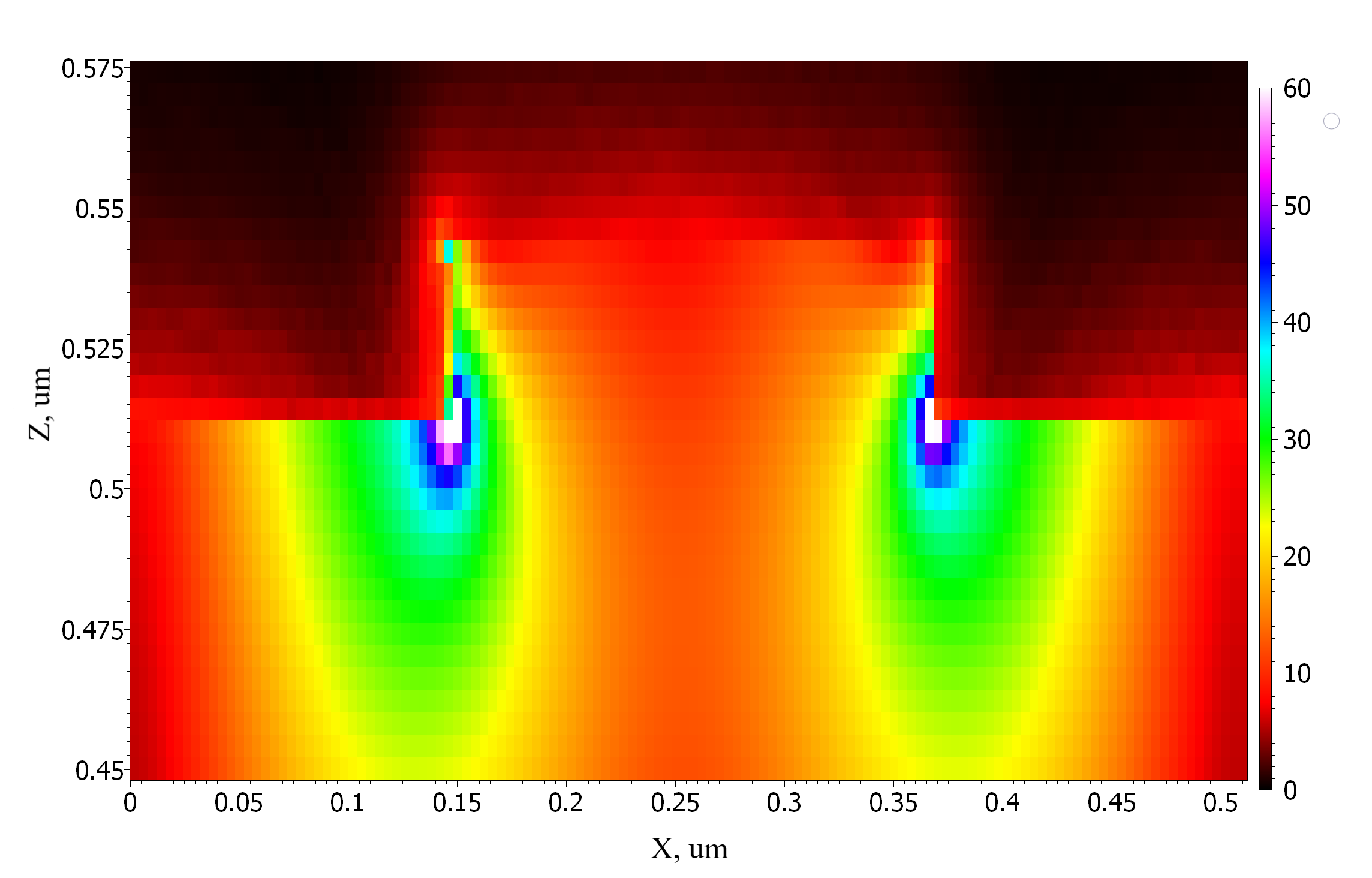
The length of the incident radiation in micrometers is plotted along the abscissa axis, and the reflection coefficient of the structure is plotted along the ordinate axis. A deep peak is visible at 556 nm. Let's construct a field distribution near the interface at a given wavelength.

The file with the field dimensions is named binary.frequency.msh. The data in it is presented in binary format and it can be opened using the program qplt. We will set the following visualization parameters of the program:

alt text

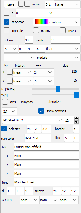
Fig. 5 Program visualization parameters qplt

distribution-of-field-2.png

Fig. 6 Modulus of electric field distribution in the structure (light fell from below). Micrometers are deposited along the OX and OZ axes, and the field module is indicated by color

On Fig. 6 bright spots are visible - these are plasmonic structures. Thanks to them, the absorption capacity of the photocathode increases dramatically, and the field is distributed optimally.

Results

Using the EMTL library, the reflection spectrum from a structure with a nanoscale one-dimensional diffraction grating was modeled. The distribution of the field at the wavelength with minimal reflection is constructed.