Mie scattering. Near field modeling

Introduction

Scattering of light by a spherical particle (Mie scattering) is a classical electrodynamic problem solved in 1908 by Gustav Mie for a spherical particle of arbitrary size. This is the problem of finding the distribution of the field when a plane wave falls on a sphere.

For particles that are much larger or much smaller than the wavelength of scattered light, there are simple and accurate approximations sufficient to describe the behavior of the system. But for objects whose size is within several orders of magnitude of the wavelength, for example, water droplets in the atmosphere, latex particles in paint, droplets in emulsions, including milk, as well as biological cells and cellular components, a more detailed approach is needed.

The following describes the process of finding the scattering efficiency spectrum and its validation. The scattering efficiency at the incidence of a plane wave is a dimensionless quantity, which is the ratio of the scattering cross-section of the body to the area of its projection on the wave front. It can be found by the formula:

\[Q_{sca} = \frac{\sigma}{S},\]

where \(\sigma\) is the scattering cross section, \(S\) is the area of the projection of the sphere onto the plane of the incident wave front. The scattering cross section can be found by the formula:

\[\sigma = \frac{W}{I\cdot S},\]

where \(W\) is the reflected flow of the field through an arbitrary closed surface, inside which there is a sphere, \(I\) is the intensity of the incident wave

fizschem.jpg

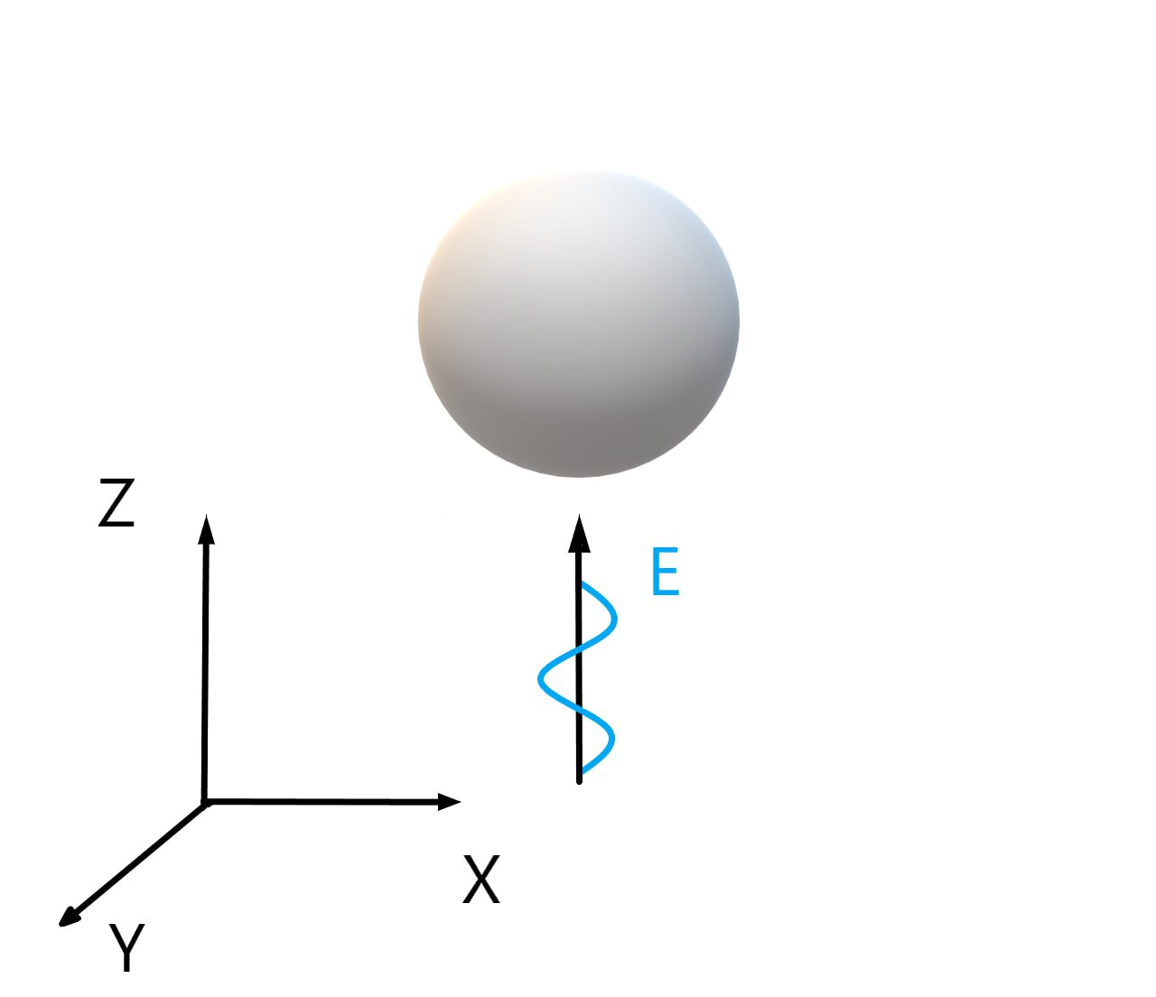
Fig. 1. Scheme of the experiment

The scheme of the physical experiment is presented in Fig. 1. The light falls in the positive direction of the OZ axis. The solitary sphere is in an unlimited volume, in which there is nothing, it is made of silver. The radius of the sphere is 128 nm

Setting up a numerical experiment

The experiment is performed in a finite wavelength range. We will indicate from 0.2 to 0.6 micrometers so that the peak of silver absorption and the effects caused by the scattering of Mie can be distinguished. Let's set the computational volume, calculations of fields are performed inside it. EMTL works on the basis of the FDTD method, so you need to set the spatial step of the grid. In order to simulate an infinite space filled with vacuum, we will establish absorbing boundary conditions. Let's add a sphere and specify its material. Let's define the Total field and Scattered field areas and the plane wave source. To find the flow of the reflected field, it is required to install flow detectors with wavelength scanning in the area of the Scattered field on a closed surface. To find the intensity of the incident wave and control the experiment, we will install point detectors that will record the amplitude of the field, in time and wave scans. Let's start the calculation by specifying the physical time of the experiment.

At the first stage of processing the results, we visualize the geometry of the experiment with all the detectors to make sure that it is constructed correctly. After that, we will plot the dependence of the amplitude of the source field on the wavelength, thus checking that the source is selected correctly. We visualize the field inside the computational volume in a time scan, checking that the calculation has not diverged. After that, we will construct the spectrum of scattering efficiency and compare it with the analytical solution, drawing conclusions about the accuracy of the calculation. Visualize the distribution of the near field. Let's investigate the convergence of the calculation by spatial resolution and make sure that it is selected correctly.

Program Description

Pict-schem.png

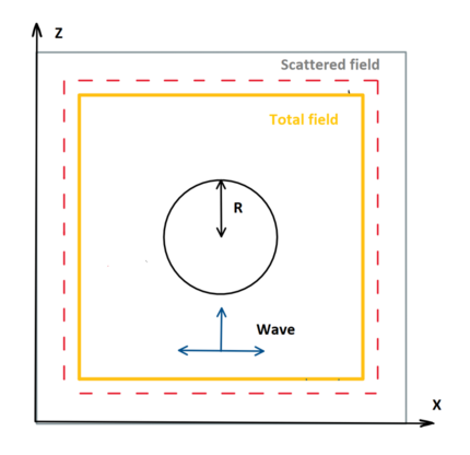
Fig. 2. The scheme of the computational experiment. The computing area is marked with a gray square, the reflected field flux detectors with a red dotted line, and the full field area with a yellow square

Stages of writing the program:

Creating a computational experiment object
Setting the program output depending on the wavelength
Specifying the wavelength range in which the spectrum will be calculated and the number of points in the spectrum
Setting the computational volume
Setting boundary conditions
Construction of the geometry of the experiment
Setting the source of a plane electromagnetic wave
Installing the detector
Starting the calculation

Processing of results:

Visualization of the scattering spectrum of a sphere
Spectrum validation with a known analytical solution
Investigation of the convergence of the scattering spectrum by spatial resolution
Visualization of the near field distribution using the program apple

To solve this problem, we will use the library EMTL, which is based on the method FDTD.

from emtl import *

EMTL performs calculations in abstract units of length, so what they will be is determined by the user. The speed of light is taken as a unit, and units of time is the period of time during which light travels a distance equal to a unit of length. Next, all units of length will be in micrometers. Let's set the radius of the sphere, the size of the computational volume, the size of the gap between the sphere and the boundaries of the computational volume, and the center of the sphere using the vector class from the EMTL library:

R = 0.128
 
additional_space_coef = 0
additional_space = R*additional_space_coef
 
x_size = 8*R+2*additional_space*R
y_size = 8*R+2*additional_space*R
z_size = 8*R+2*additional_space*R
 
center_shpere = Vector_3(x_size/2, y_size/2, z_size/2)

To correctly output the log and files, you need to connect the "sys" library and write the following command:

import sys

emInit(sys.argv[1:])

For the convenience of working with mathematical expressions, we will connect the library numpy:

import numpy as np

Sequentially, we will write a code specifying an experiment with the scattering of a plane wave on a sphere.

The FDTD experiment is carried out using the uiPyExperiment class. You need to create an object of this class, and then call its functions sequentially, with the help of which the geometry of the experiment is set, calculation and subsequent analysis are carried out. Creating an instance of the class:

task = uiPyExperiment()

For convenience, using the Use Lambda method, we will set the output of the program depending on the length of the incident wave. Now we will set the wavelength range in micrometers in which the spectrum will be calculated using the SetWavelengthRange method. The last two arguments specify the range in micrometers, and the first argument sets the upper limit of the number of points at which the spectrum will be calculated.

task.UseLambda(1)

task.SetWavelengthRange(50, 0.2, 0.6)

Setting

spatial resolution. It is selected based on the characteristic dimensions of the model, its material and the wavelength range in which the calculation is performed. To make sure that the choice of this parameter is correct, it is necessary to conduct a convergence study. Empirically, at least 15 spatial resolutions should fit on the wavelength, and at least 10 on the radius of the sphere. In this experiment, the optimal resolution is four nanometers, the convergence study on the basis of which this conclusion was made will be described below.

dx = 0.004

task.SetResolution(dx, 0.5)

The second optional argument of the SetResolution function is the Clock ratio, it is the ratio of the time step to the grid step, the default value for which is 0.5 (with this value, FDTD works steadily).

Determination of computational volume and boundary conditions

The computational volume will be a parallelepiped from (0, 0, 0) to (8*R, 8*R, 8*R). We will leave a distance of 3 radii between the sphere and the boundaries of the computational volume in order to place detectors there and leave some distance to the PML. At least one wavelength must fit between it and the material boundary:

task.SetInternalSpace(Vector_3(0), Vector_3(x_size, y_size, z_size))

We will set absorbing boundary conditions of PML in all three directions:

task.SetPMLType(NPML_TYPE)

task.SetBC(BC_PML, BC_PML, BC_PML)

We will specify the "Fourier on the fly" calculation mode using the "SetFourierOnFly" method. This allows you to speed up the program:

task.SetFourierOnFly(True)

Geometry and material definition

How to create geometric bodies is described here. If the bodies go beyond the boundaries of the computational volume, then only the part of them that falls into it is considered.

The GetSphere method sets the geometry of the sphere, taking two arguments: the radius and the coordinates of the center of the sphere:

sphere_geom = GetSphere(R, center_shpere)

FDTD does not imply the possibility of tabulating the dependence of the dielectric constant on the frequency. However, in FDTD, you can set this dependence as an arbitrary number of terms in the form of Drude and Lorentz. However, a lot of materials are already in our library. For example, using the Get A g method, you can get silver:

silver = getAg()

It remains only to add a sphere. It is important that the distance from the PML to the sphere is greater than the wavelength.

task.AddObject(silver, sphere_geom)

Total Field / Scattered Field

To generate a plane wave, we will use the Total Field/Scattered Field (TF/SF) method. TFSF technology consists in dividing space into a full field area (this is the area through which the wave from the source passes) and a scattered field area (there are no waves from the source here and therefore only reflected and scattered waves remain). At the boundary of these regions, at each time step, the fields E and H are modified according to the analytical formula. This analytical formula corresponds to the propagation of a wave of a certain type (a plane wave or a wave from a point source (dipole)). Where which area is determined for each source separately and depends on the direction of the wave it generates. The wave from the source is added (as it appears) at the border of the TFSF regions and at the next border of the TFSF regions is subtracted (disappears). The area through which it passes is called the area of the full field. The Total Field area will be located inside a parallelepiped with the coordinates of opposite vertices (R, R, R) and (7R,7R,7R).

task.AddTFSFBox(Vector_3(R), Vector_3(x_size - R, y_size - R, z_size - R))

As an incident wave used in the Total Field area, we will use a time-limited pulse with a flat front propagating in the direction (0,0,1) and polarized along the direction (1,0,0):

task.SetPlaneWave(Vector_3(0,0,1), Vector_3(1,0,0))

Detectors

In order to measure the fields inside the computational volume, detectors are needed. They read the values of the field at the points where they are placed, without affecting it in any way. The values on the detectors are obtained by interpolation over nearby grid nodes. During the numerical experiment, the detectors record their readings in binary files. Further, readable text files will be created based on these binary files.

In EMTL, there are various types of detectors that can be divided into two groups: universal and special detectors. At the same time, it is customary in EMTL to operate not with individual detectors, but with sets of detectors.

A universal detector that records the signal history in the form of a table with columns t, x, y, z, Ex, Ey, Ez, Hx, Hy, Hz for the time, coordinates and values of the fields E and H. Based on its data, for example, you can build graphs using the gnuplot program. A special detector that creates input files with time, coordinates and values of the E and H fields for plotting and 3d representation.

You can fix the flow of the reflected field using the AddFluxSet method, it creates a volume of detectors for this. This method accepts three mandatory and one optional arguments: the first argument is a string, the name of the detector group, the other two are two opposite points of the parallelipiped on the surface of which the detectors will be located, and the last and optional is the ratio of the distance between the detectors to the spatial resolution. For example, if you specify the number 1/5 as the fourth argument, then there should be one detector for 5 spatial resolutions.

det_density = 1/5

task.AddFluxSet("reflection_flux", Vector_3(round(0.5*R, 3)), Vector_3(x_size - 0.5*R, y_size - 0.5*R, z_size - 0.5*R), det_density)

Let's put an analytical detector, it will shoot the analytical waveform, that is, the E and H fields of the incident wave, such as they would be if the wave were in a vacuum. This can be done using the AddDetectorSet method by setting the DET_F | DET_SRC flags.

task.AddDetectorSet("vacuum_detector", center_shpere - Vector_3(2*R), center_shpere - Vector_3(2*R), Vector_3(1), DET_F | DET_SRC)

It is important to make sure that by the end of the calculation, the field in the computational volume has faded well (decreased in amlitude by 10 ^6 times). To do this, install the detector "E_detector" with a time sweep:

task.AddDetectorSet("E_detector", Vector_3(1.5*R), Vector_3(1.5*R), Vector_3(1))

We will also install detectors that will record the distribution of the field depending on time. To do this, install the detectors using the AddDetectorSet method. The first argument is the name of the detectors, this will also be the name of the output file for the detectors, the second and third arguments are two points specifying the parallepiped in the volume of which the detectors will be located, the fourth argumet is a vector indicating how many detectors will stand along the axes OX, OY, OZ.

task.AddDetectorSet('FILM', Vector_3(R), Vector_3(5*R),

Vector_3(round(4*R/dx, 0)), DET_BIN_ONLY)

Starting the calculation

Let's make the calculation by setting the calculation time using the Calculate method:

task.Calculate(10)

task.Analyze()

The longer the calculation time, the greater the frequency range will be calculated. The maximum frequency that the algorithm will process is given by the formula 1/t, where t is the calculation time. The first argument of the calculate method is the total calculation time. The second argument is needed when it is not necessary to calculate all frequencies in the range specified by the first argument. By specifying the second argument, you can indicate the frequency to which you want to calculate, and all the others up to the first will be filled with zeros.

Output

All files created as a result of the program can be divided into two types. The first type is files describing the model, they have extensions ".pol", ".vec", ".dat". These files are created almost immediately after the program is launched. The second type is files containing detector readings, their extensions: ".d" and ".msh". These files are created by the end of the program. A log file "proc.dat" is also created.

Files of the "first type":
"med.pol" - the file contains a description of the geometry "cell.pol" - computational volume "tf.pol" - Total Field area "sg.vec" - direction of wave movement "pmli.pol" , "pmlo.pol" - internal and external boundaries of PML files with the suffix _vset - detectors

Files of the "second type":
"reflection_flux_vset.d" - a file containing 4 columns: 1 - wavelength, 2, 3, 4 - field flow along the axis "E_detector_r0000.d" is a file containing 10 columns: 1 - time, 2, 3, 4 - detector coordinate, 6-10 - E and H fields "FILM_f****.d" - a file similar in structure "E_detector_r0000.d", only in frequency representation "binary.FILM.msh" - a file with the distribution of the field in computational volume depending on frequency, files with the extension "msh" can be opened using the built-in visualizer "qplt"

geometry-3.png

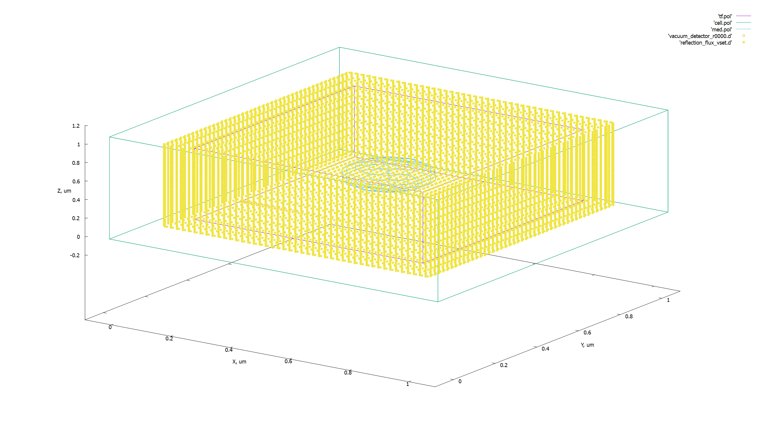
Fig. 3. Visualization of the geometry of a computational experiment using gnuplot. All values in micrometers.

Processing of results

To visualize the results, connect the libraries matplotlib and pandas:

import matplotlib.pyplot as plt

import pandas as pd

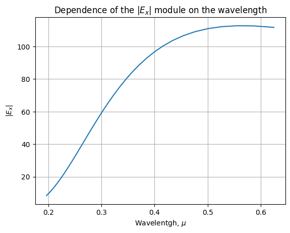
The signal must be non-zero in the wavelength range we are interested in. Let's plot the dependence of the electric field, as it would be in a vacuum, along the OX axis on the wavelength:

vacuum_field = pd.read_csv('vacuum_detector_r0000.d', sep = '\t', dtype = float)

total_field = pd.read_csv('total_field_flux.d', sep = '\t', dtype = float)

plt.plot(vacuum_field.iloc[:, 0], vacuum_field.iloc[:, 4])
plt.grid()
plt.xlabel('Wavelentgh, $\mu$')
plt.ylabel('|$E_x$|')
plt.title('Dependence of the |$E_x$| module on the wavelength')
plt.show()

png

Fig. 4. Dependence of the source field modulus on the incident wave length

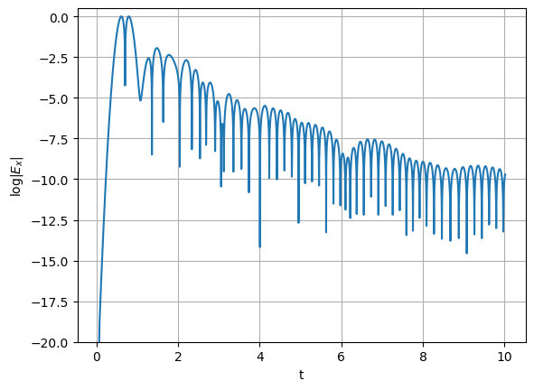
Let's make sure that the field is sufficiently attenuated. To do this, we will construct on a logarithmic scale the dependence of the field taken by the detector E_detector on time:

e_det = pd.read_csv("E_detector_r0000.d", sep = '\t', dtype = float)

plt.plot(e_det.iloc[:, 0], np.log10(e_det.iloc[:, 4]*e_det.iloc[:, 4]))
plt.grid()
plt.xlabel('t')
plt.ylabel('log|$E_x$|')
plt.ylim(-20, 0.5)
plt.show()

c:\users\mikhail\appdata\local\programs\python\python37\lib\site-packages\pandas\core\arraylike.py:364: RuntimeWarning: divide by zero encountered in log10
  result = getattr(ufunc, method)(*inputs, **kwargs)

png

Fig. 5. Dependence of the logarithm of the field modulus in computational volume on emtl time on a logarithmic scale

During the calculation, the field in the system should fade at least 1e6 times. Let's plot the dependence of the electric field modulus on time, this is Fig. 5. As you can see, the field drops 1e 8 times, so the calculation time is chosen optimally.

To calculate the intensity of the incident light, we can use the previously obtained file vacuum_detector_r0000.d, which stores the incident field in the frequency representation. Since the incident plane wave is polarized in the x direction, its intensity can be obtained as:

\[I = \left|\frac{1}{2}\cdot E_x^2\right|\]

The reflected field stream is stored in the output of the detector group reflection_flux, in the file "reflection_flux.d". To find the scattering efficiency, it is necessary to divide it by the intensity of the incident light multiplied by the area of the projection of the sphere on the front of the incident wave. The projection area of the sphere can be found from the formula:

\[S = \pi R^2\]

reflect_field = pd.read_csv('reflection_flux.d', sep = '\t', dtype = float)
 
wavelengths_range = reflect_field.iloc[:, 0]
 
vacuum_I_field = np.pi*R*R*abs(1/2*(vacuum_field.iloc[:, 4]*vacuum_field.iloc[:, 4]))
 
reflection = reflect_field.iloc[:, 1].to_numpy()/np.flip(vacuum_I_field.iloc[:].to_numpy(), 0)

Below is a comparison for \(Q_{sca}\) between EMTL and the program Mie Theory Calculator (https://nanocomposix.com/pages/mie-theory-calculator ).

data_MiTheory_calculator = pd.read_csv('mitheorycalc.csv')
 
fig, ax = plt.subplots(1, figsize = (8, 4))
 
ax.plot(data_MiTheory_calculator['Wavelength'], 1/(np.pi*R*R)*1e12*data_MiTheory_calculator['Scattering'], label = 'Mie theory', color = 'red')
ax.plot(1000*wavelengths_range, 1/2*reflection, label = 'EMTL', color = 'k')
 
ax.grid()
ax.set_xlim(200, 600)
ax.set_xlabel('Wavelength, nm')
ax.set_ylabel('$Q_{sca}$')
ax.legend()

<matplotlib.legend.Legend at 0x26a1b8fadc8>

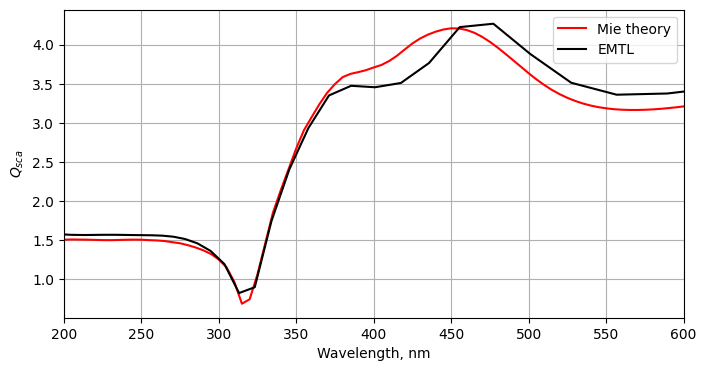
png

With the help of apple we will make a visualization (film) with the distribution of the intensity of the electric field. To do this, go to the folder where the library is stored EMTL and find a file named qplt. To the directory where qplt is located, you need to transfer the file with the movie (binary.FILM.msh). After that, enter into the command line:

python qplt binary.FILM.msh

qplt will build the movie. The viewer settings are set as in the picture below:

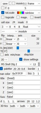
qplt_settings.jpg

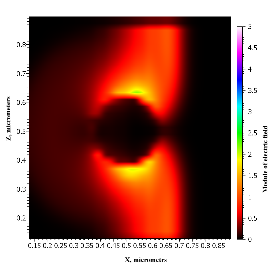
film_qplt-2.png

Fig. 6. Visualization of the near field.

Dielectric sphere

To verify the correctness of the experiment, we will construct the scattering spectrum of the glass sphere (the refractive index of the glass is 1.5). This task is easier, since you can set a smaller spatial resolution. Let's make a calculation with a spatial resolution of 16 nm and compare it with the spectrum obtained using an online calculator.

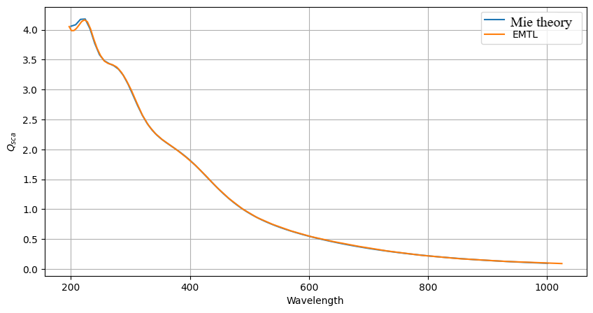
Si_comp-2.png

Fig. 7. Comparison of the scattering spectra of a glass sphere obtained using EMTL and Mie Theory Calculator. The incident wave length in nanometers is plotted along the abscissa axis, and the scattering spectrum through the cross-sectional area of the metal sphere is plotted along the ordinate axis.

The spectra match perfectly. There is a slight difference at a wavelength of 200 nm, it is due to the peculiarity of the calculation of the online calculator.

Convergence in spatial resolution

Since the geometry in the computational experiment is given discretely, the sphere cannot be represented exactly. It is extrapolated with an accuracy of the order of spatial resolution. The more optimal it is, the more optimal the approximation of the sphere is. In order to determine which spatial resolution to set, it is required to conduct a convergence study on this parameter. The result of the study is presented in Fig. 7:

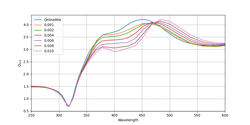
Comparing-by-dx-silver.png

Fig. 8. Investigation of convergence by spatial resolution, in the legend, the spatial resolutions of experiments are compared to the colors of the spectrum graphs, in micrometers, the incident wave length in nanometers is deposited along the abscissa axis, and scattering efficiency is plotted along the ordinate axis.

Let's calculate the discrepancy, as the average of relative errors, between the spectrum with the best spatial resolution and all the others.

\[\sigma_{dx} = \Sigma_i \left|{\frac{f_{i, dx}-f_{i, ref}}{f_{i, ref}}}\right|,\]

where \(f_{i, dx}\) is the dependence of the scattering coefficient on the incident wavelength calculated with a spatial resolution of dx nanometers, i is the wavelength number in the spectrum, \(f_{i, ref}\) is the value of the reference spectrum at the point

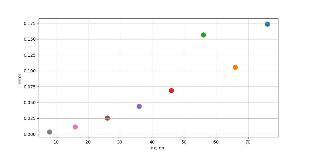
comp-by-dx.png

Fig. 9. Spatial resolution convergence study, the spatial resolution with which the experiment was carried out is postponed along the abscissa axis, and the relative error is postponed along the ordinate axis.

Based on Fig. 9, it can be concluded that convergence in spatial resolution is present and has a linear character.

Conclusion

It was shown how the EMTL library can be used to simulate the scattering of Mie. Its spectrum has been found. It describes how the geometry and modeling parameters are set in EMTL. It is indicated that the spatial resolution should be chosen based on the convergence study. Calculation time for reasons of divergence, the size of the computational domain and the optimal number of frequencies. The types of detectors are described in detail.

The stages of processing the results are described in detail, then how they can be visualized using matplotlib and gnuplot.