Transmission, reflection and absorption of light in a plane-parallel plate

Introduction

The problem of finding transmission, reflection and absorption spectra for a plane-parallel plate with finite thickness has long been solved and has a simple analytical solution. Modeling it with the EMTL library will allow you to learn the basics of the program, including setting up the dielectric properties of materials.

scheme-4.png

Problem statement

Here we will show how to calculate the reflection and transmission spectra of a gold plate.
In order to check, that we set up the simulation correctly, we will compare the simulation results with the analytical solution.

To do this, we are going to have need to write a python script for running EMTL library. Below we will describe:

how to build the geometry of the problem;
how to set the dielectric parameters of the material;
how to set up detectors in order to obtain the desired spectra;
how to visualize the results.

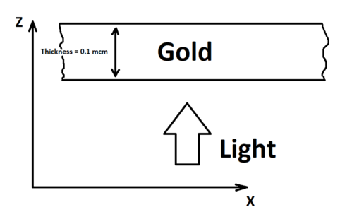
The scheme of the computational experiment can be seen in Fig. 1. The problem has a translational symmetry along two axes, so it can be considered quasi-one-dimensional. The light inpinges in the positive direction of the OZ axis on a plane-parallel plate of gold with a thickness of 50 nm. The reflection and transmission coefficients can be found by calculating the integrated reflected, transmitted and incident power fluxes. To do this, it is necessary to set up detectors that integrate the fluxes. To visualize the results, the program gnuplot and the library matplotlib are used in this example.

The spectra obtained using EMTL should be compared to the analytical solution. To do this, you need to write a simple program that will use the matrix method to calculate the spectra.

Program Description

The scheme of the numerical experiment can be seen in the picture below:

prog_scheme.png

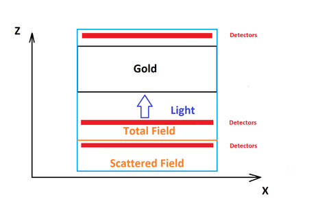
Fig. 1. The scheme of the computational experiment. The red rectangles mark the areas where the flux detectors are located, the blue rectangle is the computational volume, the yellow line is the boundary between the Total field and the Scattered field.

The light inpinges in the positive direction of the OZ axis. Detectors are marked with red rectangles. The orange line marks the border between the areas Total field and Scattered field. The blue rectangle defines the simulation domain. Finally, the black rectangle is the plate.

Preparation for the calculation

First of all, you need to import the library in your script:

import emtl

To correctly output the files, containing the simulation results, you need to import the library "sys" and write the following command:

import sys

emtl.emInit(sys.argv[1:])

For the convenience of working with mathematical expressions, we will import the library numpy:

import numpy as np

Now, let's set the thickness of the plate in micrometers:

thickness = 0.05

The FDTD experiment is carried out using the uiPyExperiment class. You need to create an object of this class, and then call its functions sequentially, with the help of which the geometry of the experiment is set, calculation and subsequent analysis are carried out. Let's create an instance of the class and specify that all results should be output depending on the wavelength:

task = emtl.uiPyExperiment()

EM performs calculations in abstract units of length, so what they will be is determined by the user. The speed of light is taken as a unit, and units of time is the period of time during which light travels a distance equal to a unit of length. For convenience, using the Use Lambda method, we will set the output of the program in wavelengths. Now we will set the wavelength range in micrometers in which the spectrum will be calculated using the SetWavelengthRange method. The last two arguments specify the range in micrometers, and the first argument sets the upper limit of the number of points at which the spectrum will be calculated.

task.UseLambda(1)

task.SetWavelengthRange(600, 0.4, 1.2)

Setting spatial resolution. It is selected based on the characteristic dimensions of the model and the wavelength range in which the calculation is performed.

dx = 0.002

task.SetResolution(dx, 0.5)

The second optional argument of the SetResolution function is the Courant ratio, it is the ratio of the time step to the grid step, the default value for which is 0.5 (with this value, FDTD scheme is stable).

The computational volume is a rectangular box stretching from (0, 0, 0) to (0, 0, 3*thickness). In front of and behind the plate, you need to leave some free space to place the detectors there:

h_space = 3*thickness

task.SetInternalSpace(emtl.Vector_3(0), emtl.Vector_3(0, 0, h_space))

Let's set absorbing PML boundary conditions on top and bottom of the computational volume and periodic conditions on the sides of the computational volume.

task.SetBC(emtl.BC_PER, emtl.BC_PER, emtl.BC_PML)

We specify the calculation mode "Fourier on the fly" using the "SetFourierOnFly" method. This allows you to speed up the program.

task.SetFourierOnFly(True)

Geometry and material definition

How to create geometric bodies is described here. If the bodies go beyond the boundaries of the computational volume, then only the part of them that falls into it is considered.

The GetPlate method sets the geometry of an infinite plate, taking three arguments: the normal vector to one of the planes bounding the plate, the coordinate of the point lying on this plane and the thickness of the plate.

plate_geom = emtl.GetPlate(emtl.Vector_3(0, 0, 1), emtl.Vector_3(0, 0, 1/3*h_space), thickness)

Definition of the material

FDTD does not imply the possibility of tabulating the dependence of the dielectric constant on the frequency. However, in FDTD, you can set this dependence as an arbitrary number of terms in the form of Drude and Lorentz. We will not dwell in detail on what parameters are set by different members, we will only give their form:

Debye: $\frac{\Delta\varepsilon}{1-2i\omega\gamma_p}$
Drude: $\frac{\Delta\varepsilon\omega_p^2}{-2i\omega\gamma_p-\omega^2}$
Lorenz: $\frac{\Delta\varepsilon \omega_p^2}{\omega_p^2-2i\omega\gamma_p-\omega^2}$
Modified Lorentz: $\frac{\Delta\varepsilon\left(\omega_p^2 - i\omega\gamma'_p\right)}{\omega_p^2-2i\omega\gamma_p-\omega^2}$

In general , the dependence of the dielectric constant on the frequency in EMTL has the form:

\[\epsilon\left(\omega\right) = \epsilon_0 + \frac{\Delta \varepsilon}{1-2i\omega\gamma_{p}} + \frac{\Delta \varepsilon \omega_{p}^2}{-2i\omega\gamma_{p}-\omega^2} + \Sigma \frac{\Delta_j \varepsilon_j \omega_{pj}^2}{\omega_{pj}^2-2i\omega\gamma_{pj}-\omega^2} + \Sigma \frac{\Delta_j \varepsilon_j \left(\omega_{pj}^2 - i\omega\gamma'_{pj}\right)}{\omega_{pj}^2-2i\omega\gamma_{pj}-\omega^2}\]

By default, a micrometer is considered a measure of length in EMTL, and the speed of light is taken as a unit, so a unit of length is the time it takes for light to travel one micrometer. The Drude-Lorentz parameters can be set in inverse seconds, electron volts, and many other systems of units. In order not to reduce them to the units accepted in the program using a calculator, there is a method calibrate

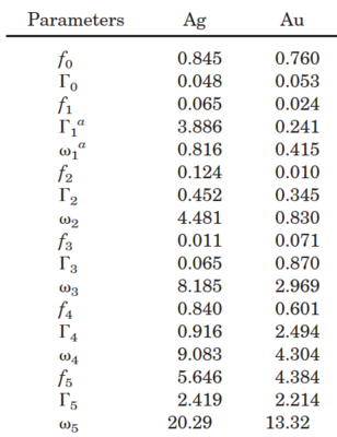
Consider the Drude-Lorentz fitting from the article A.D. Rakic et al., Applied Optics, Vol. 37, No. 22, pp. 5271-83 (1998). The fitting parameters in the article are given in the following form (in electron volts):

table_fitting.png

The permittivity dependence is given by the sum of the Drude and Lorentz terms:

\[\epsilon\left(\omega\right) = \epsilon^{(f)}\left(\omega\right) + \epsilon^{(b)}\left(\omega\right)\]

\[\epsilon^{(f)}\left(\omega\right) = 1 - \frac{\Omega_p^2}{\omega\left(\omega-i\Gamma_0\right)}\]

\[\epsilon^{(b)}\left(\omega\right) = \Sigma\frac{f_j\omega_p^2}{\left(\omega^2_j - \omega\right)+i\omega\Gamma_j}\]

We will transfer this dependency to the program by changing the parameters so that they correspond to those accepted in EMTL. In EMTL, the argument of the Lorentz term does not use a resonant frequency, but a plasma one, which means that the normalization parameter needs to be slightly changed, and the attenuation frequency is two times less:

$f'_j = \frac{\omega_{plasm}^2}{f_j^2}$
$ \Gamma' = \frac{1}{2}\cdot\Gamma$

Let's transfer this dependency to the program by changing the parameters so that they correspond to those accepted in EMTL. To do this, use the methods emMedium and AddPolarizability. The emMedium method takes the zero permittivity approximation, and AddPolarizability adds a Drude, Lorentz, Debye, or modified Lorentz term.

Method emtl.emDrude - accepts 3 arguments: plasma frequency, attenuation coefficient gamma and fitting parameter deps=1
Method emtl.emLorentz - accepts 4 arguments: plasma frequency (wp), resonance frequency, attenuation coefficient gamma and fitting parameter deps=1

To bring the parameters of the fitting to units that the program understands, you need to use the calibrate method. It multiplies all the entered dimensional parameters by its single argument. This is the coefficient of conversion of time units of dimensional parameters into time units accepted in EMTL. Let's calculate it. We will consider all lengths in EMTL to be represented in micrometers.

To find the calibration coefficient, you need to find a multiplier that allows you to convert units of time in the original system of units into units of time adopted in EMTL. In EMTL, the speed of light is considered equal to one, and the unit of length is chosen arbitrarily, we previously decided that it would be micrometers. So, the conversion factor from SI will be a unit divided by the speed of light in micrometers per second. However, the parameters in the article are set in eV, so the resulting coefficient must also be multiplied by the electron charge divided by Planck's constant. Finally, we write down the formula:

\[calibration = [\frac{e}{\hbar} \cdot \frac{1}{c}] = [\frac{e}{\hbar} \cdot \frac{1}{3e14}]\]

, where c is the speed of light in micrometers per second.

omega_plasm = 7.28
f0 = 0.760
omega0 = 0.760
gam0 = 0.043
deps0 = f0 * omega_plasm**2 / omega0**2
f1 = 0.024
omega1 = 0.335
gam1 = 0.19
deps1 = f1 * omega_plasm**2 / omega1**2
f2 = 0.010
omega2 = 0.67
gam2 = 0.28
deps2 = f2 * omega_plasm**2 / omega2**2
 
gold = emtl.emMedium(1.0)
 
gold.AddPolarizability(emtl.emDrude(f0, 1/2*gam0, deps0))
gold.AddPolarizability(emtl.emLorentz(f1, 1/2*gam1, deps1))
gold.AddPolarizability(emtl.emLorentz(f2, 1/2*gam2, deps2))
 
 
CALBR_COEF = 1.6*1e-19/(1.05*1e-34)
gold.calibrate(CALBR_COEF*1/(3e14))

Using the stack command.Dump Medium you can output a file with the values of the dielectric function. It takes two arguments: the first is the name of the file to which the output will go, and the second argument is the material whose dielectric parameters are needed.

task.DumpMedium('gold_eps', gold)

There are also a lot of materials in the built-in library:

gold = emtl.getAu()

It remains only to add the plate. Using the level parameter, you can indicate the priority of the body. The higher the value of the level attribute for a body, the higher its priority. If two bodies with different priorities overlap each other, then in the overlap region the dielectric constant will be the same as that of a body with a higher priority. By default, the body is assigned priority 0.

task.AddObject(gold, plate_geom)

Total Field / Scattered Field

To generate a plane wave, we will use the AddTFSFPlane Total Field/Scattered Field (TF/SF) method. The Total Field area will be located inside the half-space that is above the z = 0.05 plane

task.AddTFSFPlane(emtl.INF, emtl.INF, 0.05)

It is desirable that there should be a distance of at least 1.5 grid steps in space between the body and the TF/SF boundary.

As an incident wave used in the Total Field area, we will use a time-limited pulse with a flat front propagating in the direction (0,0,1) and polarized along the direction (1,0,0):

task.SetPlaneWave(emtl.Vector_3(0,0,1), emtl.Vector_3(1,0,0))

Detectors

In order to measure the fields inside the computational volume, detectors are needed. They read the values of the field at the points where they are placed, without affecting it in any way. The values on the detectors are obtained by interpolation over nearby grid nodes. During the numerical experiment, the detectors record their readings in binary files. Further, readable text files will be created based on these binary files.

The reflection coefficient can be found by dividing the reflected power flux from the structure by the power flux of the incident radiation. You can set up the detectors for calculating the reflected and transmitted power fluxes using the Addtraset method, which creates corresponding planar arrays of detectors for this. This method takes four arguments: the first argument is a string, the name of a group of detectors, the second argument is an axis that will be perpendicular to the planes of the detector arrays (detector planes) (x - 0, y - 1, z – 2), the next two arguments are the coordinates of the transmitted and reflected detector plane correspondingly. Note, that the reflected detector plane should be in the "Scattered field" region.

task.AddRTASet("flux", 2, 0.025, 2.5*thickness, thickness)

Let's make the calculation by setting the calculation time using the Calculate method:

task.Calculate(30) #first arg is time

task.Analyze()

The first argument of the Calculate method is the true time of the calculation, and the second argument is responsible for interpolation. The longer the calculation time, the more frequencies the program will be able to analyze, however, with an increase in this parameter, the calculation time of the program increases, and the probability of collisions also appears. Time is measured in inverse micrometers.

Output

All files created as a result of the program can be divided into two types. The first type is files describing the model, they have extensions ".pol", ".vec", ".dot". These files are created almost immediately after the program is launched. The second type is files containing detector readings, their extensions: ".d" and ".msh". These files are created by the end of the program. A log file "proc.dat" is also created.

Files of the "first type":

"med.pol" - the file contains a description of the geometry
"cell.pol" - computational volume
"tf.pol" - Total Field area
"sg.vec" - direction of wave movement
<- "li.pol" , "pl.pol" - internal and external boundaries of PML
<- files with the suffix _v set - detectors

Files of the "second type":

"flux.d" - a file containing 4 columns: 1 - wavelength, 2, 3, 4 - field flow along the axis

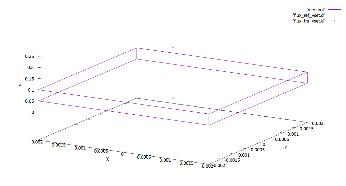
The ".pol" extension in the file name means that the polyhedron is given by the file(s) (polyhedron), the extension d is a dot (dot), and the extension ".vec" is a vector (vector). Using the program gnuplot, we build a geometry and a computational object, using the following commang: sp 'med.pol' w l, 'flux_ref_vset.d' w p, 'flux_tra_vset.d' w p

med-2.png

All values in micrometers

Let's construct the reflection spectrum of the plate. To do this, enter the command in the terminal gnuplot:

p 'flux.d' u 1:(\f$2/\f$3) w l t 'Reflectance', 'flux.d' u 1:(\f$4/\f$3) w l t 'Tansmition'

The purple curve is the output of the reflection spectrum, and the green one is the output of the transmission spectrum. Wavelentgh in micrometers

Comparison with analytics solve

The problem of the spectrum of the plate is very simple, so it has an analytical solution. To find the spectrum, we will use the matrix method.

The essence of this method is to map some matrix to each interface and environment. Our task has one plate and two interfaces. The matrix defining the interface between media with refractive indices, $n_0$ and $n_1$ is set as follows:

$A_{01}=$

\[\begin{pmatrix} \frac{n_1 + n_0}{2 \cdot n_1}& \frac{n_1 - n_0}{2 \cdot n_1}\\ \frac{n1 - n0}{2 \cdot n_1}& \frac{n_1 + n_0}{2 \cdot n_1} \end{pmatrix}\]

$F = $

\[\begin{pmatrix} e^{ikl}& 0\\ 0& e^{-ikl} \end{pmatrix}\]

$A_{10} =$

\[\begin{pmatrix} \frac{n_1 + n_0}{2 \cdot n_0}& \frac{n_0 - n_1}{2 \cdot n_0}\\ \frac{n0 - n1}{2 \cdot n_0}& \frac{n_1 + n_0}{2 \cdot n_0} \end{pmatrix}\]

Then the matrix of the system is:
\[A_{res} = A_{10}\cdot F\cdot A_{01}\]

The reflection coefficient can be found by the formula:
\[R = \left|-\frac{A_{res}^{10}}{A_{res}^{11}}\right|^2\]

, where the superscripts are the corresponding elements of the matrix of the system. To upload files to the program, connect the pandas library

import pandas as pd

import matplotlib.pyplot as plt

def Aij(n0, n1):

Aij = 1 / (2 * n1) * np.array([[n1 + n0, n1 - n0], [n1 - n0, n1 + n0]], dtype=complex)

return Aij

def Fj(k, l):

Fj = np.array([[np.exp(1.0j * k * l), 0], [0, np.exp(-1.0j * k * l)]], dtype=complex)

return Fj

data_emtl = pd.read_csv('flux.d', dtype = float, sep = '\t')

wave_lengths = data_emtl.iloc[:, 0].to_numpy()

result_refl = np.zeros((wave_lengths.shape[0], 2))

result_tra = np.zeros((wave_lengths.shape[0], 2))

Let's compare the obtained spectrum with the analytical solution. To do this, use the matrix formula. We will also write the dependence of the dielectric constant on the frequency explicitly:

for i in range(wave_lengths.shape[0]):

wave = wave_lengths[i]

eps_gold = gold.get_epsilon(2*np.pi/wave)

n_gold = np.sqrt(eps_gold)

k = 2*np.pi / wave

A_01 = Aij(1.0, n_gold)

F_1 = Fj(k*n_gold, thickness)

A_10 = Aij(n_gold, 1.0)

res_matr = np.dot(A_10, np.dot(F_1, A_01))

reflaction = -res_matr[1, 0]/res_matr[1, 1]

transmition = res_matr[0,0]+res_matr[0, 1]*reflaction

result_refl[i, 0], result_refl[i, 1] = wave, np.abs(reflaction) ** 2

result_tra[i, 0], result_tra[i, 1] = wave, np.abs(transmition) ** 2

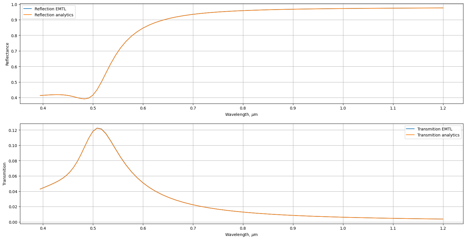
Let's compare the results of EMTL and analytics by constructing reflection and transmission spectra. To do this, we will connect the libraries matplotlib and pandas:

fig, ax = plt.subplots(2, figsize = (20, 10))

ax[0].plot(data_emtl.iloc[:, 0], data_emtl.iloc[:, 1]/data_emtl.iloc[:, 2], label = 'Reflection EMTL')

ax[0].plot(result_refl[:, 0], result_refl[:, 1], label = 'Reflection analytics')

ax[1].plot(data_emtl.iloc[:, 0], data_emtl.iloc[:, 3]/data_emtl.iloc[:, 2], label = 'Transmition EMTL')

ax[1].plot(result_tra[:, 0], result_tra[:, 1], label = 'Transmition analytics')

ax[0].legend()

ax[0].grid()

ax[0].set_xlabel('Wavelength, $\mu$m')

ax[0].set_ylabel('Reflectance')

ax[1].legend()

ax[1].grid()

ax[1].set_xlabel('Wavelength, $\mu$m')

ax[1].set_ylabel('Transmition')

plt.show()

png

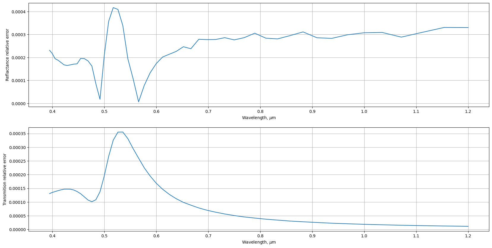
We will consider the discrepancy at a given wavelength as the modulus of difference. The spectrum of the discrepancy, the length of the incident wave in micrometers is deposited along the abscissa axis, and the absolute error of the reflection coefficient is on the ordinate axis, and in the second figure the error of the transmission coefficient.

fig, ax = plt.subplots(2, figsize = (20, 10))

ax[0].plot(data_emtl.iloc[:, 0], abs(data_emtl.iloc[:, 1]/data_emtl.iloc[:, 2] - result_refl[:, 1]))

ax[0].grid()

ax[0].set_xlabel('Wavelength, $\mu$m')

ax[0].set_ylabel('Reflactance relative error')

ax[1].plot(data_emtl.iloc[:, 0], abs(data_emtl.iloc[:, 3]/data_emtl.iloc[:, 2] - result_tra[:, 1]))

ax[1].grid()

ax[1].set_xlabel('Wavelength, $\mu$m')

ax[1].set_ylabel('Transmition relative error')

plt.show()

png

It can be seen from the graph above that the error does not exceed one thousandth. This is quite enough for the problem under consideration, but if you need to further increase the accuracy of the calculation, you can perform calculations with a better spatial resolution or set the calculation time to calculate more.

Conclusion

It was studied how to set materials using a fitting. It shows how to set the calibration. The algorithm for calculating one-dimensional structures is demonstrated in detail.