FDTD (Finite-Difference Time-Domain)

FDTD is one of the most popular numerical methods in computational electrodynamics. Since introduction in 70th years of the previous century this method became popular due to it certain advantages: simplicity of explicit numerical scheme high parallel efficiency easiness of complex geometry generation ability to handle dispersive and nonlinear media natural description of impulsive regimes

FDTD includes various numerical techniques and options, such as algorithm for dispersive and nonlinear media modeling, different mesh types, simulation results postprocessing etc.

Real optical applications often require extensive parallel FDTD calculations. One can use existing commercial solutions for this purpose, but they do not provide open code that can be modified. To cover this gap we developed Electromagnetic Template Library.

Yee algorithm

Yi's algorithm is a simple and elegant scheme for the discretization of Maxwell's equations written in differential form. The grids for the electric and magnetic fields are shifted relative to each other by half the sampling step for each of the spatial variables and in time. Finite-difference equations make it possible to determine electric and magnetic fields at a given time step based on the known values of the fields at the previous one, and under given initial conditions, the computational procedure gives an evolutionary solution in time from the beginning of the reference with a given time step.

In the absence of free charges , Maxwell 's equations in differential form have the form:

\( \frac{\partial \vec{B}}{\partial t} = -\nabla \times \vec{E} - \vec{M}, \) \( \frac{\partial \vec{D}}{\partial t} = \nabla \times \vec{H} - \vec{J}, \) \( \nabla \cdot \vec{D} = 0, \) \( \nabla \cdot \vec{B} = 0, \)

where \(\vec E\) and \(\vec H\) - electric and magnetic field strengths, \(\vec D\) - electic, \(\vec B\) - magnetic induction, \(\vec J\) - electric current density, \(\vec M\) - its magnetic counterpart, which we have included for the generality of some of the expressions used below. For the sake of simplicity of presentation, we will limit the consideration only to isotropic, non-dispersed and linear media. Then vectors \(\vec E\) and \(\vec D\), \(\vec H\) and \(\vec B\) are related by the following relations:

\( \vec{D}=\varepsilon \vec{E}=\varepsilon_r \varepsilon_0 \vec{E}, \quad \vec{B}=\mu \vec{H}=\mu_r \mu_0 \vec{H}, \)

where \(\varepsilon\), \(\varepsilon_r\), \(\mu\), \(\mu_r\) - absolute and relative dielectric and magnetic permeability of the medium, \(\varepsilon_0\) and \(\mu_0\) - electric and magnetic constants.

The density of electric and magnetic currents is represented as:

\( \vec{J}=\vec{J}_{source}+\sigma \vec{E}, \quad \vec{M}=\vec{M}_{source}+\sigma^* \vec{H}, \)

where \(\vec{J}_{source}\) - current density of free sources, \(\sigma\) - electrical conductivity, \(\vec{M}_{source}\) and \(\sigma^*\) - their magnetic counterparts.

Substituting these relations into the first pair of Maxwell's equations, we obtain

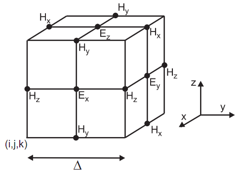
\( \frac{\partial \vec{H}}{\partial t} = -\frac{1}{\mu} \nabla \times \vec{E} - \frac{1}{\mu}\left(\vec{M}_{source} + \sigma^* \vec{H}\right), \) \( \frac{\partial \vec{E}}{\partial t} = \frac{1}{\varepsilon}\nabla \times \vec{H} - \frac{1}{\varepsilon}\left(\vec{J}_{source} + \sigma \vec{E}\right). \)

According to the algorithm And, Maxwell's equations are discretized using a central difference relation to approximate the spatial and temporal derivatives. To do this, the grid nodes in which the components of the electric and magnetic fields are stored are shifted relative to each other by half a grid step for each of the spatial variables. As a result, those nodes that correspond to the components of the fields \(\vec{E}\) are arranged in such a way that each component \(\vec E\) is surrounded by four components \(\vec H\), and vice versa.

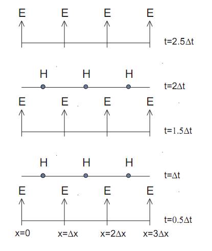
The positions of grid nodes for electric and magnetic field components on the Yi grid.

According to the Yi algorithm, the nodes corresponding to the components \(\vec E\) and \(\vec H\) are shifted relative to each other in time by half a time step (as an example, this is demonstrated below for a one-dimensional Yi grid). To calculate the values of the field \(\vec E\) on the \(n+1/2\)th time step, the values of the field \(\vec H\) on the \(n\)th are used. Similarly, the values of the field \(\vec H\) at \(n+1\)th step are calculated using the values of the field \(\vec E\) at \(n+1/2\)th step. This procedure continues until the calculation is completed.

Scanning of the one-dimensional Yi grid in time: the nodes corresponding to the electric and magnetic fields are shifted relative to each other in space and time by half a step.

Before getting the specific difference equations used in the Yi algorithm, we introduce the following notation. We will match each grid node with three integers \(i\), \(j\) and \(k\), defining the position of this node in space as

\( (i,j,k)=(i\Delta x,j\Delta y,k\Delta z), \)

where \(\Delta x\), \(\Delta y\) and \(\Delta z\) are the grid steps in the corresponding directions. We will denote an arbitrary grid function \(u\) as

\( u(i \Delta x, j \Delta y, k \Delta z, n \Delta t)=u_{i,j,k}^n, \)

where \(\Delta t\) is the time step, and \(n\) is the current time step.

As already mentioned, Yi's algorithm uses a central difference relation to approximate the derivatives present in Maxwell's equations. So, for the derivative of the coordinate \(x\) at the point \((i\Delta x, j\Delta y, k\Delta z)\) at the time \(n \Delta t\) we have

\( \frac{\partial u}{\partial x}(i \Delta x, j \Delta y, k \Delta z, n \Delta t)=\frac{u_{i+1/2,j,k}^n-u_{i-1/2,j,k}^n}{\Delta x}+O\left[(\Delta x)^2\right]. \)

Similarly for the time derivative \(t\)

\( \frac{\partial u}{\partial t}(i \Delta x, j \Delta y, k \Delta z, n \Delta t)=\frac{u_{i,j,k}^{n+1/2}-u_{i,j,k}^{n-1/2}}{\Delta t}+O\left[(\Delta t)^2\right]. \)

Applying these approximations for derivatives involved in the projection of Ampere's law on the \(x\) axis

\( \frac{\partial E_x}{\partial t}=\frac{1}{\varepsilon} \left[ \frac{\partial H_z}{\partial y} - \frac{\partial H_y}{\partial z} - \left(J_{source,x}+\sigma E_x\right)\right], \)

we get

\( \varepsilon_{i,j+1/2, k+1/2}\frac{E_x|_{i,j+1/2, k+1/2}^{n+1/2}-E_x|_{i,j+1/2, k+1/2}^{n-1/2}}{\Delta t}= \) \( \frac{H_z|_{i,j+1, k+1/2}^n-H_z|_{i,j, k+1/2}^n}{\Delta y} -\frac{H_y|_{i,j+1/2, k+1}^n-H_y|_{i,j+1/2, k}^n}{\Delta z} -J_x|_{i,j+1/2, k+1/2}^n - \sigma_{i,j+1/2, k+1/2}E_x|_{i,j+1/2, k+1/2}^n. \)

The variables on the right side are taken at the time step \(n\), including the field \(E_x\). Since there is no data on the grid for the value \(E_x\) at the time \(n\), you need to use some kind of approximation for it. Averaging over adjacent time layers is a good choice.:

\( E_x|_{i,j+1/2, k+1/2}^n=\frac{E_x|_{i,j+1/2, k+1/2}^{n+1/2}+E_x|_{i,j+1/2, k+1/2}^{n-1/2}}{2}. \)

Let \(\Delta=\Delta x=\Delta y=\Delta z\). Then we can explicitly express \(E_x\) by \(n+1/2\) step:

\( E_x|_{i,j+1/2, k+1/2}^{n+1/2}= C_{a,E_x}|_{i,j+1/2, k+1/2} E_x|_{i,j+1/2, k+1/2}^{n-1/2} + \) \( C_{b,E_x}|_{i,j+1/2, k+1/2} ( H_z|_{i,j+1, k+1/2}^n-H_z|_{i,j, k+1/2}^n + H_y|_{i,j+1/2, k}^n-H_y|_{i,j+1/2, k+1}^n - J_x|_{i,j+1/2, k+1/2}^n \Delta ), \)

where

\( C_{a}|_{i,j,k}=\left( 1-\frac{\sigma_{i,j,k}\Delta t}{2 \varepsilon_{i,j,k}} \right)\left( 1+\frac{\sigma_{i,j,k}\Delta t}{2 \varepsilon_{i,j,k}} \right)^{-1}, \) \( C_{b}|_{i,j,k}=\left( \frac{\Delta t}{\varepsilon_{i,j,k} \Delta} \right)\left( 1+\frac{\sigma_{i,j,k}\Delta t}{2 \varepsilon_{i,j,k}} \right)^{-1}. \)

We have obtained a difference equation corresponding to the projection of Ampere's law on the \(x\) axis, which together with the five remaining similar difference equations form the Yi algorithm.

It can be shown that in the case of a non-conducting medium ( \(\sigma=0\)) and in the absence of current sources \(\vec{J}\), the two Maxwell equations remaining unused by us are executed automatically, namely, the divergence of fields \(\vec{E}\) and \(\vec{H}\) are always zero. In the presence of current sources, the validity of the two remaining equations does not follow directly from the difference scheme, but is confirmed with good accuracy in a numerical experiment.

The choice of values \(\Delta x\), \(\Delta y\), \(\Delta z\) is determined by the geometry of the problem and the spectral composition of the radiation. You can give the following recommendation: the characteristic size of the object (the radius of the balls, the thickness of the screen, etc.) should account for at least several grid steps, and the characteristic wavelength - from ten or more. The magnitude of the value \(\Delta t\) is bounded from above by the Courant condition

\( \Delta t<\frac{1}{c\sqrt{\displaystyle{\frac{1}{(\Delta x)}^2+\frac{1}{(\Delta y)^2}+\frac{1}{(\Delta z)^2}}}}, \)

the implementation of which is necessary for the stability of the difference scheme.

In this section we have considered the implementation of the Yi algorithm for the case when the medium is characterized by frequency-independent scalar values \(\varepsilon\), \(\mu\), \(\sigma\), \(\sigma^*\). Numerical modeling of anisotropic, dispersed and nonlinear media requires modification of this algorithm and application of auxiliary difference equations.

Note also that the numerical scheme FDTD does not imply the possibility of tabular determination of the dependence of the dielectric constant on the frequency. How to model dispersed materials in FDTD, you can read in the section HTTPS.

Next part is here: FDTD numerical experiment