FDTD numerical experiment
Typical scenario of FDTD experiment includes following steps: User specifies calculated volume and mesh resolution, optical properties and geometry of the structure, boundary conditions (typically, periodic or absorbing), wave source and set of points where field values should be recorded (we call it detectors). Source generates finite time width impulse impinging on structure. Its propagation and scattering is recorded by detectors and possibly transformed to the frequency domain. Total exit of the radiation through absorbing boundaries determines the simulation time. Recorded field values are processed (for example, energy flux integrating through the chosen surface) to get optical characteristics of the structure.
The usual scenario of a numerical experiment FDTD looks like this:
- Inside the computational volume set by the size of the grid used, material bodies, the source and detectors are placed (detectors are not answered by any real bodies in space, they only mean that we write the values of the fields at some points in a file). Boundary conditions, usually periodic or absorbing, should be set at the boundary of the computational volume.
- The source generates a finite electromagnetic wave in time, the spectral composition of which should cover the frequency range of interest to us. Further, the wave falls on the bodies, disperses onto them, and, in the presence of absorbing boundary conditions, after some time leaves the computational volume. The history of wave propagation is recorded by detectors.
- Using the Fourier transform, the field values recorded on the detectors are translated into a frequency representation. Further, by processing them (for example, integrating the energy flow of the field through any surface), we obtain the optical characteristics of the structure of the bodies in question that interest us.
Let's explain some of the concepts we used.
Absorbing boundary conditions
To eliminate the non-physical re-reflection of the electromagnetic wave from the boundary of the computational volume and thus simulate the departure of the wave to infinity in FDTD, special absorbing boundary conditions should be used. Currently, the most successful implementation of these conditions is the placement of a thin layer of special material called a Perfectly Matched Layer (PML) along the boundary of the computational volume. Ideally, this material completely absorbs all waves incident on it without any reflection, regardless of the angle of incidence and wavelength.
The concept of a perfectly matched layer (PML) was introduced by J.-P. Berenger in 1994. The work of such a layer was based on splitting the initial fields \(\vec E\) and \(\vec H\) into two components, for each of which its own equations should be solved. Subsequently, improved formulations of PML equivalent to Berenger's original formulation were proposed. Thus, Uniaxial PML uses an anisotropic absorbing material, which makes it possible not to introduce additional variables and remain within the framework of the original Maxwell equations. However, uniaxial PML, as well as PML in Berenger's formulation, are not convenient because there is no absorption of damped waves in them, which does not allow placing PML close to scattering bodies. This disadvantage is deprived of the revolving PML (Convolutional PML), based on the analytical continuation of Maxwell's equations into the complex plane in such a way that their solution exponentially decays. CPML is also more convenient in limiting infinite conductive and dispersed media. In addition, the mathematical formulation of CPML has greater clarity and accessibility for understanding.
In some cases, the use of PML leads to FDTD divergence. This problem can be fixed by using the Additional back absorbing layers technique HTTPS PDF
Periodic boundary conditions
FDTD can be used not only for finite, but also for infinite periodic structures. Periodic boundary conditions in one or several directions are used for their modeling. In particular, photonic crystal plates and anti-reflective coatings are planar periodic structures: they are periodic in two directions and have a limited length in the remaining direction. Real experimental samples, of course, have a limited size in the first two directions, but since this size is significantly larger than their length in the non-periodic direction, the influence of the finiteness of the sample with a good degree of accuracy can be neglected.
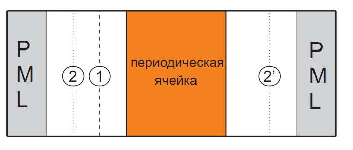
In practical applications, as a rule, the transmission and reflection spectra from the structures under consideration are the most interesting. To obtain them in the case of a normal fall in FDTD, the following numerical experiment is used. The boundary between the regions of the full and scattered fields generates a plane wave in the form of a time-limited pulse that falls on the structure (in the figure below, this pulse is generated at the boundary 1 and moves from left to right). Part of the incident pulse is reflected from the structure, crosses the plane in which the detectors measuring the reflected wave are located (plane 2 in the figure), and is absorbed by the PML back layer. The other part passes through the structure, crosses the plane in which the detectors measuring the transmitted wave are located (plane 2' in the figure), and is absorbed by the front layer of PML. The numerical experiment continues until the signal leaves the computational volume. The signal output time depends on the specific geometry of the experiment. With an increase in the longitudinal length of the structure, this time increases due to an increase in the distance that the signal must travel to get out of it. The signal output time also depends on the optical properties of the structure under study, for example, in the presence of absorption, it is less.
At the end of the experiment, the values of the fields \(\vec E(t)\), \(\vec H(t)\) recorded by the detectors are translated into a frequency representation using a discrete Fourier transform. Next, calculating the average value of the Poynting vector in time \(\vec S(\omega)\) on each of the detectors according to the formula
we can calculate the average energy flow \(W(\omega)\) passing through the surface \(A\) on which the detectors are located:
By normalizing the energy flow of the transmitted and reflected wave to the incident pulse, we obtain the transmission spectra of \(T(\omega) that interest us\) and reflections \(R(\omega)\). Absorption is calculated as \(A(\omega)=1-T(\omega)-R(\omega)\).
The FDTD scheme for modeling the oblique incidence of a plane wave on a periodic structure can be found here HTTPS, PDF
Subgrid smoothing method
As in any other difference method, in FDTD there is a problem of inaccurate mapping of the body boundary to the computational grid. In the immediate vicinity of the boundary of the two media, Maxwell's equations must be solved taking into account the boundary conditions for the vectors \(\vec E\) and \(\vec H\). Any curved surface separating neighboring media and geometrically inconsistent with the grid will be distorted by the "ladder approximation" effect. As a result, the order of accuracy of the FDTD is lowered from the original second to the first.
Various methods have been proposed to solve this problem. The first group of methods is based on changing the method of discretization of Maxwell's equations in order for the grid to correspond to the geometry under consideration as much as possible. For example, one of these methods is to increase the resolution of the grid in those areas of space where bodies with a complex geometric structure are located. It is also possible to modify the difference equations in the grid nodes located near the boundary between neighboring bodies. A more radical step is the introduction of an irregular non-orthogonal grid that would be completely consistent with the geometry in question. Such a grid is automatically generated by a program that monitors the placement of all bodies in space. A common disadvantage of these methods is an increase in the amount of memory required and sometimes a significant decrease in performance.
Another group of methods is based on the introduction of an effective permittivity \(\varepsilon\) near the boundary between bodies. Consider some control volume \({\delta}x\times{\delta}y\times{\delta}z\) surrounding the selected grid node, and assume that it contains the interface between two media with permittivity values \(\varepsilon_1\) and \(\varepsilon_2\). Then the boundary conditions for the vectors \(\vec{E}\) and \(\vec{D}\) can be implemented on the grid by entering the inverse permittivity tensor in the form:
where \({\bf P}\) is the matrix \(P_{ij}=n_in_j\) corresponding to the projector on the normal vector \(\vec{n}\) to the boundary between the two media, and \(<>\) is averaging by volume.
You can read more about the implementation of this method in FDTD here HTTPS, PDF
Next read here: Using FDTD